The Boundary Conditions

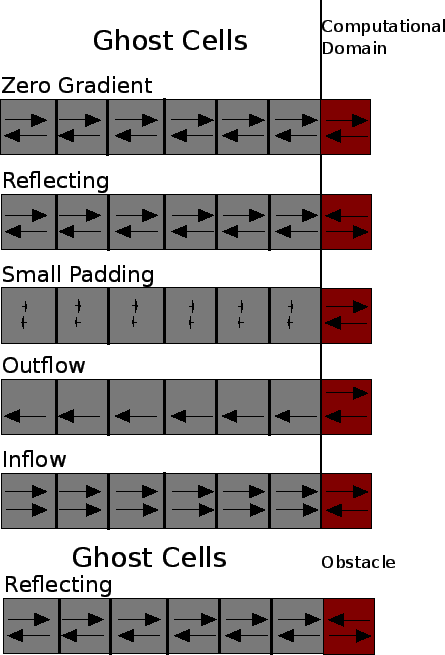
TYCHO comes with five different boundary conditions to choose from, namely Zero Gradient, Reflecting, Small Number Padding, Outflow, Inflow and Periodic. These boundary conditions can be attached separately to all edges of the computational domain. The exact definition of the conditions can be found in the file set_boundary.c. In Fig. 3.1 the handling of the velocity vector for all different boundary conditions is given. In the case of the Small Padding boundary conditions the density, pressure and total energy is set to small (i.e. 1.0E-50) values in the ghost cells. The other boundary conditions copy density, pressure and total energy in the ghost cells, as defined in set_boundary.c . A special behavior is implemented for the Inflow/Outflow boundary conditions. In the first case a constant inflow of gas with a velocity, density and temperature specified in the Parameterfile is realized and in the second case gas which leaves the computational domain will not enter it again, because backflow of gas is prevented.
In the case of obstacles in the computational domain TYCHO will split the calculations into two parts, i.e. boundary at the computational domain and boundary at the obstacles. The boundaries at the obstacles are always reflecting.
In the following example source section taken from set_boundary.c, the handling of the left and right edges of the computational domain are shown. In principle one can easily implement own boundary conitions in the same way. The integers nmin and nmax stand for the first and last cells in the gas part of the computational domain. TYCHO has six ghost cells for the PPM Method. The arrays dx, xa, dx0 and xa0 contain the spacing and the positions of the left faces of the cells in code units.

/*!
 Reflecting boundary condition
 */
int left_boundary_reflecting(int nmin, int nmax,
    double *rho_1D, double *eng_1D, double *pre_1D,
    double *vx_1D, double *vy_1D, double *vz_1D,
    double *xa0, double *dx0, double *xa, double *dx,
    int flag) {

    int n;

    for (n = 1; n < 7; n++) {
        rho_1D[nmin - n] = rho_1D[nmin + n - 1];
        pre_1D[nmin - n] = pre_1D[nmin + n - 1];
        eng_1D[nmin - n] = eng_1D[nmin + n - 1];

        vx_1D[nmin - n] = -1 * vx_1D[nmin + n - 1];
        vy_1D[nmin - n] = -1 * vy_1D[nmin + n - 1];
        vz_1D[nmin - n] = -1 * vz_1D[nmin + n - 1];

        dx[nmin - n] = dx[nmin + n - 1];
        xa[nmin - n] = xa[nmin - n + 1] - dx[nmin - n];
        dx0[nmin - n] = dx0[nmin + n - 1];
        xa0[nmin - n] = xa0[nmin - n + 1] - dx0[nmin - n];
    }

    return 0;
}

/*!
 Reflecting boundary condition
 */
int right_boundary_reflecting(int nmin, int nmax,
    double *rho_1D, double *eng_1D, double *pre_1D,
    double *vx_1D, double *vy_1D, double *vz_1D,
    double *xa0, double *dx0, double *xa, double *dx,
    int flag) {
    int n;

    for (n = 1; n < 7; n++) {
        rho_1D[n + nmax] = rho_1D[nmax + 1 - n];
        pre_1D[n + nmax] = pre_1D[nmax + 1 - n];
        eng_1D[n + nmax] = eng_1D[nmax + 1 - n];

        vx_1D[n + nmax] = -vx_1D[nmax + 1 - n];
        vy_1D[n + nmax] = -vy_1D[nmax + 1 - n];
        vz_1D[n + nmax] = -vz_1D[nmax + 1 - n];

        dx[n + nmax] = dx[nmax + 1 - n];
        xa[n + nmax] = xa[nmax + n - 1] + dx[nmax + n - 1];
        dx0[n + nmax] = dx0[nmax + 1 - n];
        xa0[n + nmax] = xa0[nmax + n - 1] + dx0[nmax + n - 1];
    }

    return 0;
}

Figure 3.1: The handling of the velocities for the differnent implemented boundary conditions at the left edge of the computational domain.