The Sod Shock-Tube in 1D

The Sod shock tube problem, named after Gary A. Sod, is a test for the accuracy of the Riemann solver. In Fig. 9.1 and 9.2 the initial conditions for the 1D case are shown. The initial conditions are set up as defined here

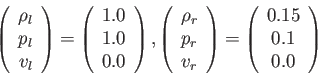$$\left(\begin{array}{c} \rho_l\\ p_{l}\\ v_l\end{array}\right... ...t) = \left(\begin{array}{c} 0.15\\ 0.1\\ 0.0\end{array}\right)$$ (9.1)

After 0.2s the solution of the density and pressure are shown in Fig. 9.3 and Fig. 9.4. The typical regions are clearly visible, i.e. the rarefaction wave, the contact discontinuity and the shock discontinuity. More information on this test scenario can be found at
http://en.wikipedia.org/wiki/Sod_shock_tubehttp://en.wikipedia.org/wiki/Sod_shock_tube.

Figure 9.1: The initial conditions for the 1D Sod Shock-Tube problem (density distribution shown).

Figure 9.2: The initial conditions for the 1D Sod Shock-Tube problem (pressure distribution shown).

Figure 9.3: The 1D Sod Shock-Tube problem after 0.2 s of evolution. The density of the gas is shown.

Figure 9.4: The 1D Sod Shock-Tube problem after 0.2 s of evolution. The pressure of the gas is shown.